3 Population Ecology
Caralyn Zehnder, Kalina Manoylov, Samuel Mutiti, Christine Mutiti, Allison VandeVoort, Donna Bennett
Population Ecology
Ecology is a sub-discipline of biology that studies the interactions between organisms and their environments. A group of interbreeding individuals (individuals of the same species) living and interacting in a given area at a given time is defined as a population. These individuals rely on the same resources and are influenced by the same environmental factors. Population ecology, therefore, is the study of how individuals of a particular species interact with their environment and change over time. The study of any population usually begins by determining how many individuals of a particular species exist, and how closely associated they are with each other. Within a particular habitat, a population can be characterized by its population size (N), defined by the total number of individuals, and its population density, the number of individuals of a particular species within a specific area or volume (units are number of individuals/unit area or unit volume). Population size and density are the two main characteristics used to describe a population. For example, larger populations may be more stable and able to persist better than smaller populations because of the greater amount of genetic variability, and their potential to adapt to the environment or to changes in the environment. On the other hand, a member of a population with low population density (more spread out in the habitat), might have more difficulty finding a mate to reproduce compared to a population of higher density. Other characteristics of a population include dispersion – the way individuals are spaced within the area; age structure – number of individuals in different age groups and; sex ratio – proportion of males to females; and growth – change in population size (increase or decrease) over time.
Exponential Growth
Charles Darwin, in his theory of natural selection, was greatly influenced by the English clergyman Thomas Malthus. Malthus published a book (An Essay on the Principle of Population) in 1798 stating that populations with unlimited natural resources grow very rapidly. According to the Malthus’ model, once population size exceeds available resources, population growth decreases dramatically. This accelerating pattern of increasing population size is called exponential growth, meaning that the population is increasing by a fixed percentage each year. When plotted (visualized) on a graph showing how the population size increases over time, the result is a J-shaped curve (Figure 3.1). Each individual in the population reproduces by a certain amount (r) and as the population gets larger, there are more individuals reproducing by that same amount (the fixed percentage). In nature, exponential growth only occurs if there are no external limits.
One example of exponential growth is seen in bacteria. Bacteria are prokaryotes (organisms whose cells lack a nucleus and membrane-bound organelles) that reproduce by fission (each individual cell splits into two new cells). This process takes about an hour for many bacterial species. If 100 bacteria are placed in a large flask with an unlimited supply of nutrients (so the nutrients will not become depleted), after an hour, there is one round of division and each organism divides, resulting in 200 organisms – an increase of 100. In another hour, each of the 200 organisms divides, producing 400 – an increase of 200 organisms. After the third hour, there should be 800 bacteria in the flask – an increase of 400 organisms. After a day and 12 of these cycles, the population would have increased from 100 cells to more than 24,000 cells. When the population size, N, is plotted over time, a J-shaped growth curve is produced (Figure 3.1). This shows that the number of individuals added during each reproduction generation is accelerating – increasing at a faster rate.
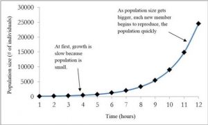
Figure 3.1: The “J” shaped curve of exponential growth for a hypothetical population of bacteria. The population starts out with 100 individuals and after 11 hours there are over 24,000 individuals. As time goes on and the population size increases, the rate of increase also increases (each step up becomes bigger). In this figure “r” is positive.
Per capita rate of increase (r)
In exponential growth, the population growth rate (G) depends on population size (N) and the per capita rate of increase (r). In this model r does not change (fixed percentage) and change in population growth rate, G, is due to change in population size, N. As new individuals are added to the population, each of the new additions contribute to population growth at the same rate (r) as the individuals already in the population.
r = (birth rate + immigration rate) – (death rate and emigration rate).
If r is positive (> zero), the population is increasing in size; this means that the birth and immigration rates are greater than death and emigration.
If r is negative (< zero), the population is decreasing in size; this means that the birth and immigration rates are less than death and emigration rates.
If r is zero, then the population growth rate (G) is zero and population size is unchanging, a condition known as zero population growth. “r” varies depending on the type of organism, for example a population of bacteria would have a much higher “r” than an elephant population. In the exponential growth model r is multiplied by the population size, N, so population growth rate is largely influenced by N. This means that if two populations have the same per capita rate of increase (r), the population with a larger N will have a larger population growth rate than the one with a smaller N.
Logistic Growth
Exponential growth cannot continue forever because resources (food, water, shelter) will become limited. Exponential growth may occur in environments where there are few individuals and plentiful resources, but soon or later, the population gets large enough that individuals run out of vital resources such as food or living space, slowing the growth rate. When resources are limited, populations exhibit logistic growth. In logistic growth a population grows nearly exponentially at first when the population is small and resources are plentiful but growth rate slows down as the population size nears limit of the environment and resources begin to be in short supply and finally stabilizes (zero population growth rate) at the maximum population size that can be supported by the environment (carrying capacity). This results in a characteristic S-shaped growth curve (Figure 3.2). The mathematical function or logistic growth model is represented by the following equation:
Where, K is the carrying capacity – the maximum population size that a particular environment can sustain (“carry”). Notice that this model is similar to the exponential growth model except for the addition of the carrying capacity.
In the exponential growth model, population growth rate was mainly dependent on N so that each new individual added to the population contributed equally to its growth as those individuals previously in the population because per capita rate of increase is fixed. In the logistic growth model, individuals’ contribution to population growth rate depends on the amount of resources available (K). As the number of individuals (N) in a population increases, fewer resources are available to each individual. As resources diminish, each individual on average, produces fewer offspring than when resources are plentiful, causing the birth rate of the population to decrease.
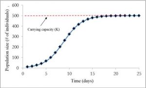
Figure 3.2: Shows logistic growth of a hypothetical bacteria population. The population starts out with 10 individuals and then reaches the carrying capacity of the habitat which is 500 individuals.
Yeast is a microscopic fungus, used to make bread and alcoholic beverages, that exhibits the classical S-shaped logistic growth curve when grown in a test tube (Figure 3.3). Its growth levels off as the population depletes the nutrients that are necessary for its growth. In the real world, however, there are variations to this idealized curve. For example, a population of harbor seals may exceed the carrying capacity for a short time and then fall below the carrying capacity for a brief time period and as more resources become available, the population grows again (Figure 3.4). This fluctuation in population size continues to occur as the population oscillates around its carrying capacity. Still, even with this oscillation, the logistic model is exhibited.
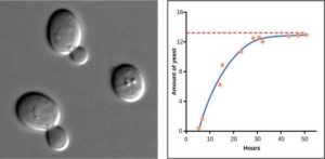
Figure 3.3: Graph showing amount of yeast versus time of growth in hours. The curve rises steeply, and then plateaus at the carrying capacity. Data points tightly follow the curve. The image is a micrograph (microscope image) of yeast cells
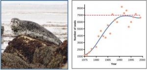
Figure 3.4: Graph showing the number of harbor seals versus time in years. The curve rises steeply then plateaus at the carrying capacity, but this time there is much more scatter in the data. A photo of a harbor seal is shown.
Factors limiting population growth
Recall previously that we defined density as the number of individuals per unit area. In nature, a population that is introduced to a new environment or is rebounding from a catastrophic decline in numbers may grow exponentially for a while because density is low and resources are not limiting. Eventually, one or more environmental factors will limit its population growth rate as the population size approaches the carrying capacity and density increases. Example: imagine that in an effort to preserve elk, a population of 20 individuals is introduced to a previously unoccupied island that’s 200 km2 in size. The population density of elk on this island is 0.1 elk/km2 (or 10 km2 for each individual elk). As this population grows (depending on its per capita rate of increase), the number of individuals increases but the amount of space does not so density increases. Suppose that 10 years later, the elk population has grown to 800 individuals, density = 4 elk/ km2 (or 0.25 km2 for each individual). The population growth rate will be limited by various factors in the environment. For example, birth rates may decrease due to limited food or death rate increase due to rapid spread of disease as individuals encounter one another more often. This impact on birth and death rate in turn influences the per capita rate of increase and how the population size changes with changes in the environment. When birth and death rates of a population change as the density of the population changes, the rates are said to be density-dependent and the environmental factors that affect birth and death rates are known as density-dependent factors. In other cases, populations are held in check by factors that are not related to the density of the population and are called density-independent factors and influence population size regardless of population density. Conservation biologists want to understand both types because this helps them manage populations and prevent extinction or overpopulation.
The density of a population can enhance or diminish the impact of density-dependent factors. Most density-dependent factors are biological in nature (biotic), and include such things as predation, inter- and intraspecific competition for food and mates, accumulation of waste, and diseases such as those caused by parasites. Usually, higher population density results in higher death rates and lower birth rates. For example, as a population increases in size food becomes scarcer and some individuals will die from starvation meaning that the death rate from starvation increases as population size increases. Also as food becomes scarcer, birth rates decrease due to fewer available resources for the mother meaning that the birth rate decreases as population size increases. For density-dependent factors, there is a feedback loop between population density and the density-dependent factor.
Two examples of density-dependent regulation are shown in Figure 3.5. First one is showing results from a study focusing on the giant intestinal roundworm (Ascaris lumbricoides), a parasite that infects humans and other mammals. Denser populations of the parasite exhibited lower fecundity (number of eggs per female). One possible explanation for this is that females would be smaller in more dense populations because of limited resources and smaller females produce fewer eggs.
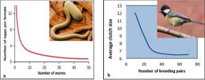
Figure 3.5: (a) Graph of number of eggs per female (fecundity), as a function of population size. In this population of roundworms, fecundity (number of eggs) decreases with population density, (b) Graph of clutch size (number of eggs per “litter”) of the great tits bird as a function of population size (breeding pairs). Again, clutch size decreases as population density increases. (Photo credits: Worm image from Wikimedia commons, public domain image; bird image from Wikimedia commons, photo by Francis C. Franklin / CC-BY-SA-3.0)
Density-independent birth rates and death rates do NOT depend on population size; these factors are independent of, or not influenced by, population density. Many factors influence population size regardless of the population density, including weather extremes, natural disasters (earthquakes, hurricanes, tornadoes, tsunamis, etc.), pollution and other physical/abiotic factors. For example, an individual deer may be killed in a forest fire regardless of how many deer happen to be in the forest. The forest fire is not responding to deer population size. As the weather grows cooler in the winter, many insects die from the cold. The change in weather does not depend on whether there is a population size of 100 mosquitoes or 100,000 mosquitoes, most mosquitoes will die from the cold regardless of the population size and the weather will change irrespective of mosquito population density. Looking at the growth curve of such a population would show something like an exponential growth followed by a rapid decline rather than levelling off (Figure 3.6).
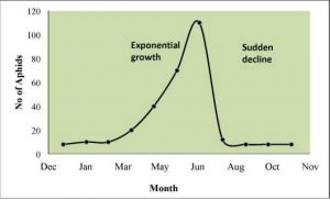
Figure 3.6: Weather change acting as a density-independent factor limiting aphid population growth. This insect undergoes exponential growth in the early spring and then rapidly die off when the weather turns hot and dry in the summer
In real-life situations, density-dependent and independent factors interact. For example, a devastating earthquake occurred in Haiti in 2010. This earthquake was a natural geologic event that caused a high human death toll from this density-independent event. Then there were high densities of people in refugee camps and the high density caused disease to spread quickly, representing a density-dependent death rate.
